Lemurs

Author

Adaobi Nwankwo

Lemurs Analysis

I’m choosing to work on this data set from the Duke Lemur Center.

Loading Packages and Data sets

Reading in the data. Here we will load the tidyverse package and Lemurs data.

#Load the tidyverse
library(tidyverse)
── Attaching packages ─────────────────────────────────────── tidyverse 1.3.2 ──
✔ ggplot2 3.4.0      ✔ purrr   1.0.0 
✔ tibble  3.1.8      ✔ dplyr   1.0.10
✔ tidyr   1.2.1      ✔ stringr 1.5.0 
✔ readr   2.1.3      ✔ forcats 0.5.2 
── Conflicts ────────────────────────────────────────── tidyverse_conflicts() ──
✖ dplyr::filter() masks stats::filter()
✖ dplyr::lag()    masks stats::lag()
library(kableExtra)

Attaching package: 'kableExtra'

The following object is masked from 'package:dplyr':

    group_rows
lemurs <- readr::read_csv('https://raw.githubusercontent.com/rfordatascience/tidytuesday/master/data/2021/2021-08-24/lemur_data.csv')
Rows: 82609 Columns: 54
── Column specification ────────────────────────────────────────────────────────
Delimiter: ","
chr  (19): taxon, dlc_id, hybrid, sex, name, current_resident, stud_book, es...
dbl  (27): birth_month, litter_size, expected_gestation, concep_month, dam_a...
date  (8): dob, estimated_concep, dam_dob, sire_dob, dod, weight_date, conce...

ℹ Use `spec()` to retrieve the full column specification for this data.
ℹ Specify the column types or set `show_col_types = FALSE` to quiet this message.
#install.packages("tidymodels")
library(tidymodels)
── Attaching packages ────────────────────────────────────── tidymodels 1.0.0 ──
✔ broom        1.0.2     ✔ rsample      1.1.1
✔ dials        1.1.0     ✔ tune         1.0.1
✔ infer        1.0.4     ✔ workflows    1.1.2
✔ modeldata    1.1.0     ✔ workflowsets 1.0.0
✔ parsnip      1.0.3     ✔ yardstick    1.1.0
✔ recipes      1.0.4     
── Conflicts ───────────────────────────────────────── tidymodels_conflicts() ──
✖ scales::discard()        masks purrr::discard()
✖ dplyr::filter()          masks stats::filter()
✖ recipes::fixed()         masks stringr::fixed()
✖ kableExtra::group_rows() masks dplyr::group_rows()
✖ dplyr::lag()             masks stats::lag()
✖ yardstick::spec()        masks readr::spec()
✖ recipes::step()          masks stats::step()
• Search for functions across packages at https://www.tidymodels.org/find/
my_data_splits <- initial_split(lemurs, prop = 0.5)

exploratory_data <- training(my_data_splits)
test_data <- testing(my_data_splits)
#install.packages("skimr")
library(skimr)
exploratory_data%>%
  skim()
Data summary
Name Piped data
Number of rows 41304
Number of columns 54
_______________________
Column type frequency:
character 19
Date 8
numeric 27
________________________
Group variables None

Variable type: character

skim_variable n_missing complete_rate min max empty n_unique whitespace
taxon 0 1.00 3 4 0 27 0
dlc_id 0 1.00 3 4 0 2012 0
hybrid 0 1.00 1 2 0 2 0
sex 0 1.00 1 2 0 3 0
name 0 1.00 2 19 0 1991 0
current_resident 0 1.00 1 1 0 2 0
stud_book 1389 0.97 1 7 0 1145 0
estimated_dob 36008 0.13 1 3 0 8 0
birth_type 0 1.00 2 3 0 3 0
birth_institution 0 1.00 8 44 0 83 0
dam_id 521 0.99 3 9 0 545 0
dam_name 7622 0.82 2 15 0 466 0
dam_taxon 7622 0.82 3 4 0 27 0
sire_id 865 0.98 3 9 0 471 0
sire_name 12431 0.70 2 17 0 395 0
sire_taxon 12431 0.70 3 4 0 26 0
dob_estimated 36008 0.13 1 3 0 8 0
age_category 0 1.00 2 11 0 3 0
preg_status 0 1.00 1 2 0 2 0

Variable type: Date

skim_variable n_missing complete_rate min max median n_unique
dob 3 1.00 1958-10-01 2018-07-24 1994-03-20 1403
estimated_concep 3 1.00 1958-06-03 2018-05-22 1993-10-26 1434
dam_dob 7622 0.82 1958-10-01 2014-09-13 1986-06-26 409
sire_dob 12431 0.70 1946-10-01 2014-08-07 1985-11-29 358
dod 18698 0.55 1969-06-02 2019-01-15 2008-12-02 1192
weight_date 0 1.00 1968-09-16 2019-02-05 2005-12-19 8848
concep_date_if_preg 40358 0.02 1971-11-09 2018-05-22 2003-09-09 497
infant_dob_if_preg 40358 0.02 1972-03-08 2018-07-24 2004-02-16 489

Variable type: numeric

skim_variable n_missing complete_rate mean sd p0 p25 p50 p75 p100 hist
birth_month 3 1.00 5.57 2.70 1.00 4.00 5.00 7.00 12.00 ▇▇▇▂▃
litter_size 9048 0.78 1.65 0.82 1.00 1.00 1.00 2.00 4.00 ▇▅▁▂▁
expected_gestation 0 1.00 119.58 39.73 62.00 90.00 124.00 160.00 193.00 ▆▃▇▅▂
concep_month 3 1.00 6.63 3.69 1.00 4.00 6.00 11.00 12.00 ▆▆▃▂▇
dam_age_at_concep_y 7625 0.82 7.17 4.62 0.59 3.63 6.38 10.16 26.03 ▇▆▂▁▁
sire_age_at_concep_y 12434 0.70 9.11 6.28 0.61 4.62 7.44 12.37 33.36 ▇▅▂▁▁
age_at_death_y 18701 0.55 17.50 8.50 0.00 11.04 17.34 23.42 39.39 ▃▇▇▅▂
age_of_living_y 26771 0.35 13.50 8.93 0.54 6.60 10.65 19.81 35.20 ▇▇▃▃▂
age_last_verified_y 37139 0.10 12.61 8.09 0.36 6.71 10.08 18.55 34.26 ▆▇▃▃▂
age_max_live_or_dead_y 3 1.00 15.60 8.87 0.00 7.79 14.46 22.65 39.39 ▇▇▆▅▂
n_known_offspring 18315 0.56 5.62 4.77 1.00 2.00 4.00 7.00 36.00 ▇▂▁▁▁
weight_g 0 1.00 1479.33 1308.11 4.74 199.00 1300.00 2480.00 10245.00 ▇▅▁▁▁
month_of_weight 0 1.00 6.50 3.39 1.00 4.00 7.00 9.00 12.00 ▇▆▆▆▇
age_at_wt_d 3 1.00 3087.62 2829.28 0.00 744.00 2285.00 4791.00 14373.00 ▇▃▂▁▁
age_at_wt_wk 3 1.00 441.09 404.18 0.00 106.29 326.43 684.43 2053.29 ▇▃▂▁▁
age_at_wt_mo 3 1.00 101.51 93.02 0.00 24.46 75.12 157.51 472.54 ▇▃▂▁▁
age_at_wt_mo_no_dec 3 1.00 101.02 93.01 0.00 24.00 75.00 157.00 472.00 ▇▃▂▁▁
age_at_wt_y 3 1.00 8.46 7.75 0.00 2.04 6.26 13.13 39.38 ▇▃▂▁▁
change_since_prev_wt_g 1137 0.97 20.00 173.60 -1760.00 -20.00 2.00 47.00 3662.00 ▁▇▁▁▁
days_since_prev_wt 1137 0.97 54.90 151.37 0.00 13.00 28.00 55.00 7113.00 ▇▁▁▁▁
avg_daily_wt_change_g 1247 0.97 0.56 11.51 -920.00 -0.63 0.13 1.79 300.00 ▁▁▁▇▁
days_before_death 18698 0.55 2710.07 2281.73 0.00 860.00 2120.00 4084.00 13052.00 ▇▃▂▁▁
r_min_dam_age_at_concep_y 0 1.00 1.56 0.91 0.40 0.79 1.53 1.76 4.22 ▆▇▂▁▁
expected_gestation_d 40358 0.02 141.59 33.58 62.00 124.00 145.00 165.00 193.00 ▂▂▇▇▅
days_before_inf_birth_if_preg 40358 0.02 67.57 47.25 0.00 26.00 62.00 104.00 193.00 ▇▆▅▃▁
pct_preg_remain_if_preg 40358 0.02 0.48 0.31 0.00 0.20 0.48 0.76 1.00 ▇▆▆▆▆
infant_lit_sz_if_preg 40361 0.02 1.31 0.61 1.00 1.00 1.00 1.00 4.00 ▇▂▁▁▁

Here, I loaded in a data set for the exploratory data of the Lemur data set. This is half of the data set.

exploratory_data %>%
  head(10) %>%
  kable() %>%
  kable_styling(c("hover", "striped"))
taxon dlc_id hybrid sex name current_resident stud_book dob birth_month estimated_dob birth_type birth_institution litter_size expected_gestation estimated_concep concep_month dam_id dam_name dam_taxon dam_dob dam_age_at_concep_y sire_id sire_name sire_taxon sire_dob sire_age_at_concep_y dod age_at_death_y age_of_living_y age_last_verified_y age_max_live_or_dead_y n_known_offspring dob_estimated weight_g weight_date month_of_weight age_at_wt_d age_at_wt_wk age_at_wt_mo age_at_wt_mo_no_dec age_at_wt_y change_since_prev_wt_g days_since_prev_wt avg_daily_wt_change_g days_before_death r_min_dam_age_at_concep_y age_category preg_status expected_gestation_d concep_date_if_preg infant_dob_if_preg days_before_inf_birth_if_preg pct_preg_remain_if_preg infant_lit_sz_if_preg
PCOQ 6727 N F Antonia N 178 1998-02-22 2 NA CB Duke Lemur Center 1 160 1997-09-15 9 6398 PAULINA PCOQ 1991-01-24 6.65 6450 VALENTINIAN PCOQ 1991-11-02 5.87 2017-05-23 19.26 NA NA 19.26 4 NA 5500 2002-09-18 9 1669 238.43 54.87 54 4.57 -70 15 -4.67 5361 2.64 young_adult NP NA NA NA NA NA NA
NCOU 1958 N F RANI N 1403 1989-03-17 3 NA CB Duke Lemur Center 1 193 1988-09-05 9 1903 LALITA NCOU 1985-04-08 3.41 993 KALKI NCOU 1984-05-03 4.35 2009-01-09 19.83 NA NA 19.83 2 NA 1336 1995-07-05 7 2301 328.71 75.65 75 6.30 41 34 1.21 4937 1.33 adult NP NA NA NA NA NA NA
LTAR 1921 N F ASHWANI N 1067 1986-12-23 12 NA CB Duke Lemur Center 1 167 1986-07-09 7 991 KIRAN LTAR 1982-04-12 4.24 990 RAJIV LTAR 1982-04-12 4.24 2005-08-09 18.64 NA NA 18.64 3 NA 165 2000-03-02 3 4818 688.29 158.40 158 13.20 0 38 0.00 1986 0.99 adult NP NA NA NA NA NA NA
DMAD 6451 N M Mephistopheles N 114 1981-10-08 10 Y01 WB Madagascar / NA 165 1981-04-26 4 WILD NA NA NA NA WILD NA NA NA NA 2014-02-12 32.37 NA NA 32.37 7 Y01 2790 2003-12-09 12 8097 1156.71 266.20 266 22.18 10 8 1.25 3718 4.22 adult NP NA NA NA NA NA NA
GMOH 3141 N F SEAGRAPE N NA 1989-02-01 2 NA CB Duke Lemur Center 2 124 1988-09-30 9 3099 LYSILOMA GMOH 1987-03-22 1.53 3104 VIRBURNAM GMOH 1987-05-12 1.39 1998-09-24 9.65 NA NA 9.65 3 NA 147 1996-06-05 6 2681 383.00 88.14 88 7.35 -3 28 -0.11 841 0.40 adult NP NA NA NA NA NA NA
MMUR 7047 N M Spalt Y 727 2011-06-07 6 NA CB Duke Lemur Center 3 63 2011-04-05 4 7028 Calendula MMUR 2008-05-25 2.86 MULT2 NA NA NA NA NA NA 7.67 NA 7.67 NA NA 71 2014-09-26 9 1207 172.43 39.68 39 3.31 -3 7 -0.43 NA 0.59 adult NP NA NA NA NA NA NA
EFUL 6123 N F Frigga N 1075 1984-03-31 3 NA CB BREC's Baton Rouge Zoo NA 120 1983-12-02 12 3532 LIBYA EFUL 1977-06-27 6.44 556 CADMUS EFUL 1970-03-15 13.73 2014-01-22 29.83 NA NA 29.83 1 NA 3040 2005-07-21 7 7782 1111.71 255.85 255 21.32 0 10 0.00 3107 1.39 adult NP NA NA NA NA NA NA
MZAZ 360 N M MONJO N 146 1987-04-21 4 NA CB Duke Lemur Center 2 90 1987-01-21 1 318 FANDRASA MZAZ 1979-08-25 7.41 319 GAKA MZAZ 1979-08-25 7.41 2002-11-20 15.59 NA NA 15.59 3 NA 345 2000-01-04 1 4641 663.00 152.58 152 12.72 -10 29 -0.34 1051 0.82 adult NP NA NA NA NA NA NA
MMUR 7032 N M Pesto Y 718 2008-06-04 6 NA CB Museum National d'Histoire Naturelle NA 63 2008-04-02 4 oi_162A NA NA NA NA oi_149I NA NA NA NA NA NA 10.68 NA 10.68 6 NA 72 2018-10-24 10 3794 542.00 124.73 124 10.39 1 15 0.07 NA 0.59 adult NP NA NA NA NA NA NA
MZAZ 2310 N M KIKIMOVA N 205 1993-08-02 8 NA CB Duke Lemur Center 2 90 1993-05-04 5 321 PITSY MZAZ 1982-09-02 10.68 315 AROSY MZAZ 1979-08-25 13.70 2010-02-03 16.52 NA NA 16.52 NA NA 219 1994-03-09 3 219 31.29 7.20 7 0.60 1 6 0.08 5810 0.82 IJ NP NA NA NA NA NA NA

Introduction

This data comes from the Duke Lemur Center. The Duke Lemur Center houses over 200 lemurs across 14 species. Lemurs are the most threatened group of mammals and are at risk of extinction. Lemurs are native to Madagascar which is located in the southwestern Indian Ocean. This data set contains taxonomic code, specimen ID, hybrid status, sex, name, DOB, birth month, birth type, birth institution, litter size, and many more interesting variables about lemurs. This is a very large data set containing several different variables.

Abstract

This is a very large data set so the purpose of asking these questions is to find interesting hypotheses to ask. Exploring the data will make it easier to create hypotheses. Here are some interesting questions I asked.

  • How many Lemurs are there? By sex?
  • What is the average weight of a Lemur? What about for each taxon?
  • What is the average birth type for a Lemur? By sex? By Taxon?
  • Does average litter size change by birth type?

In this report, these questions will be answered using different functions and visuals. An hypothesis will also be created and functions and visuals will support or refute the hypothesis. The purpose of this research is to shed light on Lemurs because I feel like Lemurs as a whole aren’t really talked about much. The outcomes of this research will provide us with a lot more knowledge about Lemurs and their lifestyle.

Hypotheses

  1. If hybrid Lemurs are born then they are more likely to be captive-born rather than wild-born.

  2. If Lemurs are mating it will more likely be in April and then the infants will be born around August and September.

Answering Our Questions

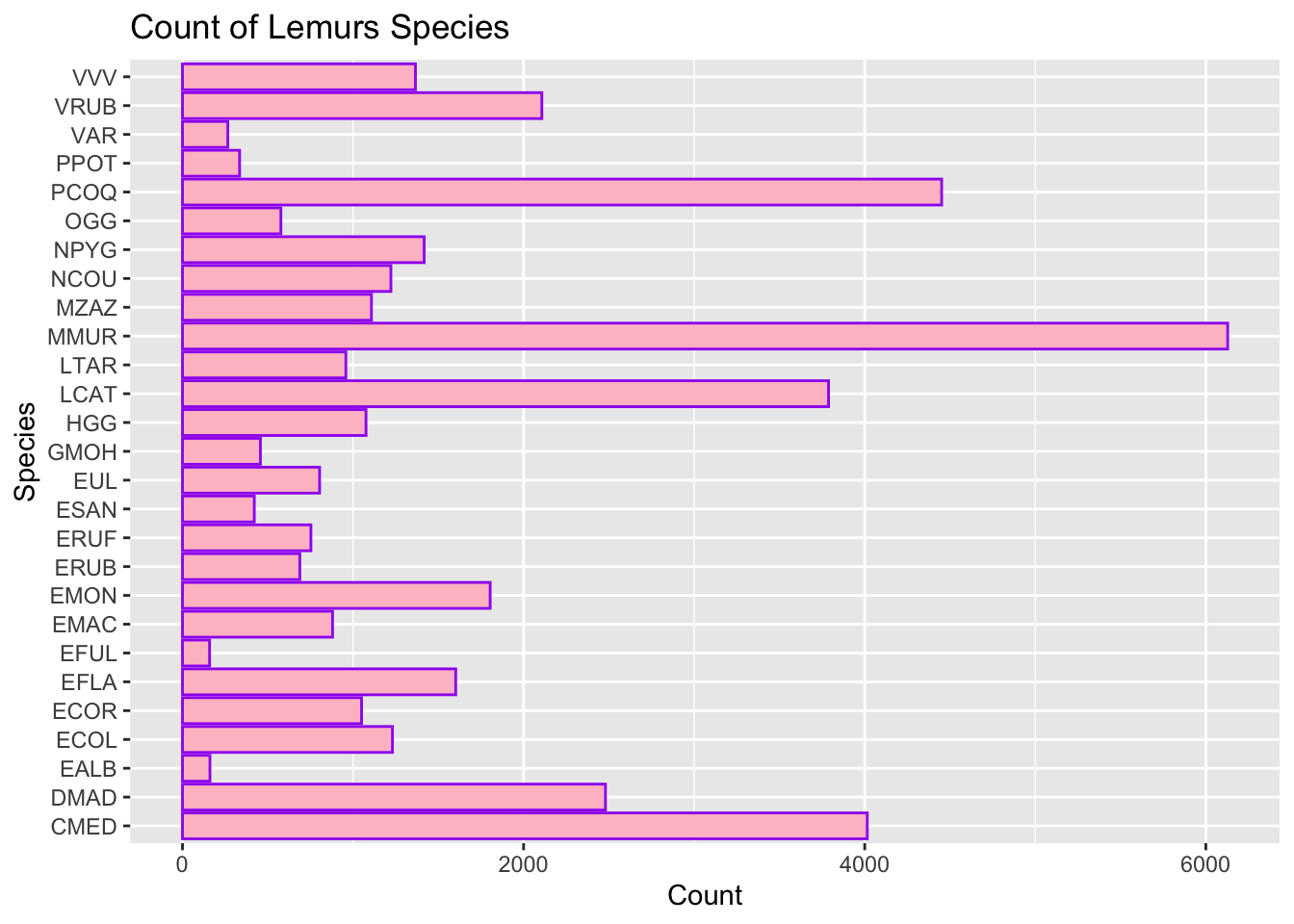
Here we will look at the number of Lemurs in the data set and separate them by sex. We will also see the Lemurs grouped by their name. It is evident that there are 41,305 Lemurs within this data set. Out of these, 20,179 are female, 21,117 are male, and 8 are not determined. In is evident that in the table and the graph, MMUR has the biggest species count, with a count of 6,127.

exploratory_data %>%
  count(sex)
# A tibble: 3 × 2
  sex       n
  <chr> <int>
1 F     20349
2 M     20948
3 ND        7
exploratory_data %>%
  count(taxon)
# A tibble: 27 × 2
   taxon     n
   <chr> <int>
 1 CMED   4015
 2 DMAD   2480
 3 EALB    161
 4 ECOL   1231
 5 ECOR   1050
 6 EFLA   1602
 7 EFUL    159
 8 EMAC    880
 9 EMON   1804
10 ERUB    688
# … with 17 more rows
exploratory_data %>%
  count(name)
# A tibble: 1,991 × 2
   name         n
   <chr>    <int>
 1 AARON        1
 2 ABAS         9
 3 ABDUL        2
 4 ABEDNIGO    13
 5 ABEL         2
 6 ABENA       51
 7 ABIGAIL      2
 8 ABSINTHE     2
 9 Abu        116
10 ACHILLES     1
# … with 1,981 more rows
exploratory_data %>%
  group_by(name) %>%
  count(sex)
# A tibble: 1,992 × 3
# Groups:   name [1,991]
   name     sex       n
   <chr>    <chr> <int>
 1 AARON    M         1
 2 ABAS     M         9
 3 ABDUL    M         2
 4 ABEDNIGO M        13
 5 ABEL     M         2
 6 ABENA    F        51
 7 ABIGAIL  F         2
 8 ABSINTHE M         2
 9 Abu      F       116
10 ACHILLES M         1
# … with 1,982 more rows
exploratory_data %>%
  ggplot() +
  geom_bar(mapping = aes(x = taxon), color = "purple", fill = "pink") +
  labs(title ="Count of Lemurs Species", x = "Species", y = "Count") +
coord_flip()

Here we will see the average weight of a Lemur. To narrow this even more, we will look at the average weight of a Lemur per taxon. After running this, it is evident that the average weight of a Lemur is 1,484.9 grams. This is about 3.3 pounds which is very light. The taxon MMUR (Gray Mouse Lemur) has the lightest weight of 74 grams or 0.16 pounds. The taxon EFUL (Common Brown Lemur) has the heaviest weight of 2,372 grams or about 5 pounds.

exploratory_data %>%
  summarize(avg_lemur_weight = mean(weight_g))
# A tibble: 1 × 1
  avg_lemur_weight
             <dbl>
1            1479.
exploratory_data %>%
  group_by(taxon) %>%
  summarize(avg_lemur_weight = mean(weight_g))
# A tibble: 27 × 2
   taxon avg_lemur_weight
   <chr>            <dbl>
 1 CMED              208.
 2 DMAD             2179.
 3 EALB             2092.
 4 ECOL             2285.
 5 ECOR             1484.
 6 EFLA             2134.
 7 EFUL             2321.
 8 EMAC             2221.
 9 EMON             1427.
10 ERUB             2105.
# … with 17 more rows

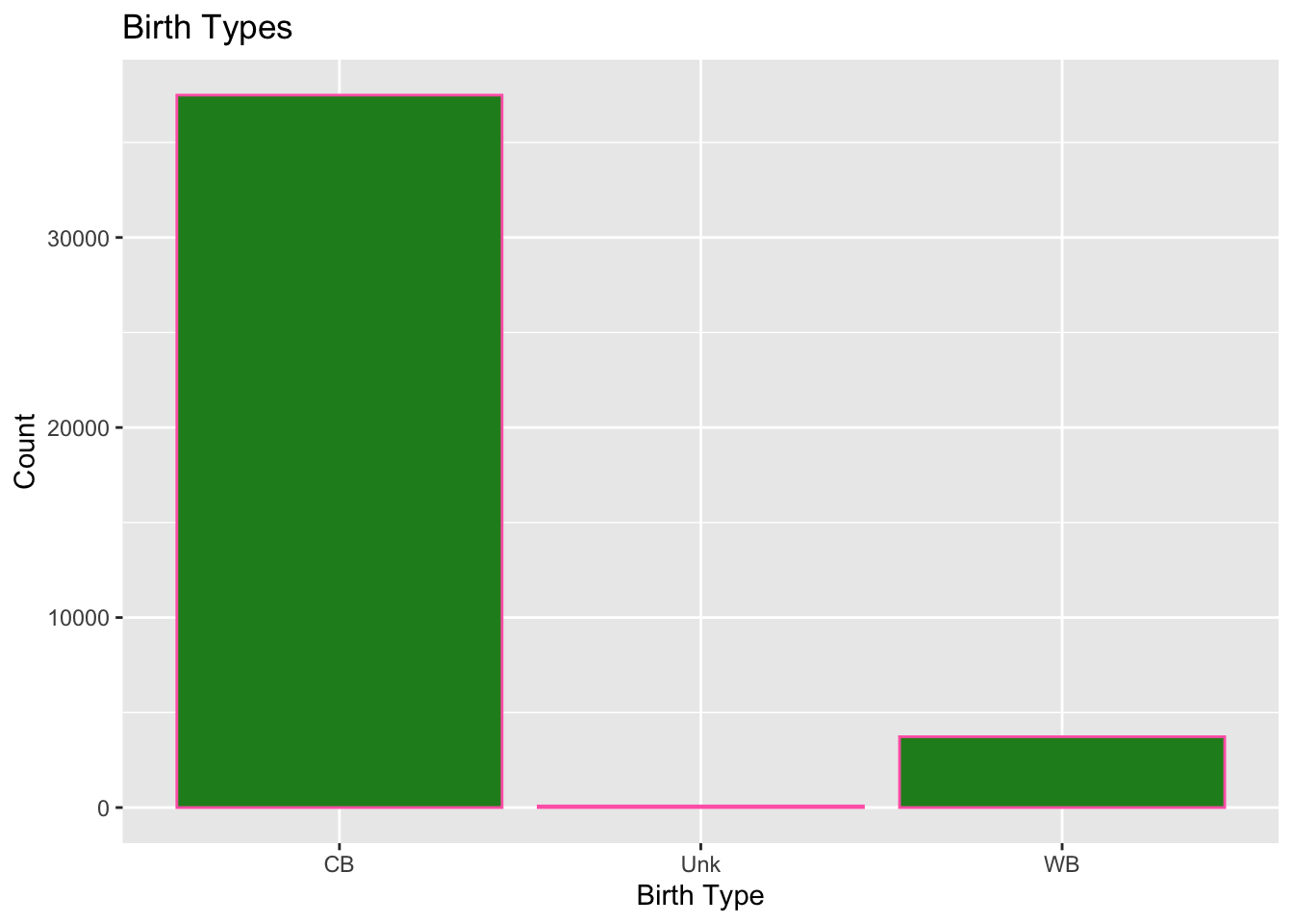
Using the exploratory data it is evident that a larger majority are captive born. 37,489 are captive born while 3,724 are wild born. This may be because Lemurs are becoming extinct so it is harder for them to be born in the wild with larger numbers. When looking at birth type through taxon, it is evident that there are very few taxon that are wild born. When looking at sex, there is not a large gap between the different birth types when looking at sex. These variables are split pretty evenly. The graph shows the amount of birth types and it is very evident that the bar for captive born surpasses the bar for wild born by a large gap.

exploratory_data %>%
  count(birth_type)
# A tibble: 3 × 2
  birth_type     n
  <chr>      <int>
1 CB         37491
2 Unk           85
3 WB          3728
exploratory_data %>%
  group_by(taxon) %>%
  count(birth_type)
# A tibble: 55 × 3
# Groups:   taxon [27]
   taxon birth_type     n
   <chr> <chr>      <int>
 1 CMED  CB          4013
 2 CMED  WB             2
 3 DMAD  CB          1541
 4 DMAD  WB           939
 5 EALB  CB           161
 6 ECOL  CB          1122
 7 ECOL  WB           109
 8 ECOR  CB           998
 9 ECOR  Unk            6
10 ECOR  WB            46
# … with 45 more rows
exploratory_data %>%
  group_by(sex) %>%
  count(birth_type)
# A tibble: 7 × 3
# Groups:   sex [3]
  sex   birth_type     n
  <chr> <chr>      <int>
1 F     CB         18350
2 F     Unk           59
3 F     WB          1940
4 M     CB         19134
5 M     Unk           26
6 M     WB          1788
7 ND    CB             7
exploratory_data %>%
  ggplot() +
  geom_bar(mapping = aes(x = birth_type), color = "hotpink", fill = "forestgreen") +
  labs(title ="Birth Types", x = "Birth Type", y = "Count")

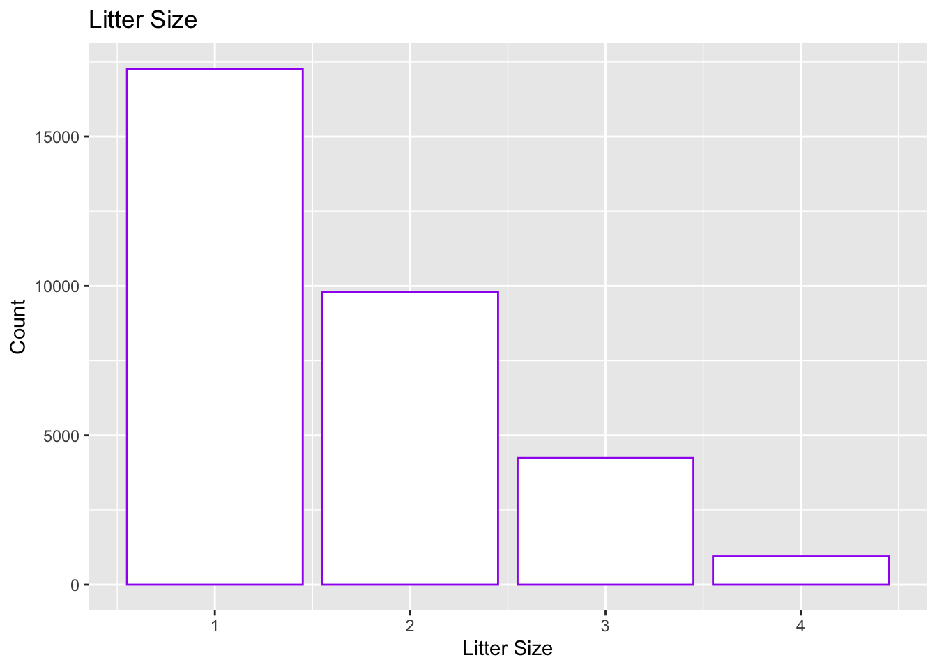
It is evident that the average litter size is 1 with a count of 17,296. As the litter size goes up to 2, 3, and 4 it becomes more unlikely. A litter size of 4 has a count of 925. This could be another reason why Lemurs are becoming extinct. Since the litter size is lower, there is a lower number of species being born which correlates with the reduced population as a whole. Looking at the data regarding litter size and birth type it is evident that there is no data regarding the litter size of wild born Lemurs. This makes sense because it would be harder and maybe even impossible to track the litter size of wild born Lemurs.

exploratory_data %>%
  count(litter_size)
# A tibble: 5 × 2
  litter_size     n
        <dbl> <int>
1           1 17267
2           2  9804
3           3  4241
4           4   944
5          NA  9048
exploratory_data %>%
  ggplot() +
  geom_bar(mapping = aes(x = litter_size), color = "purple", fill = "white") +
  labs(title ="Litter Size", x = "Litter Size", y = "Count")
Warning: Removed 9048 rows containing non-finite values (`stat_count()`).

exploratory_data %>%
  group_by(birth_type) %>%
  count(litter_size)
# A tibble: 7 × 3
# Groups:   birth_type [3]
  birth_type litter_size     n
  <chr>            <dbl> <int>
1 CB                   1 17267
2 CB                   2  9804
3 CB                   3  4241
4 CB                   4   944
5 CB                  NA  5235
6 Unk                 NA    85
7 WB                  NA  3728

Answering Our Hypothesis

  1. If hybrid Lemurs are born then they are more likely to be captive-born rather than wild-born.

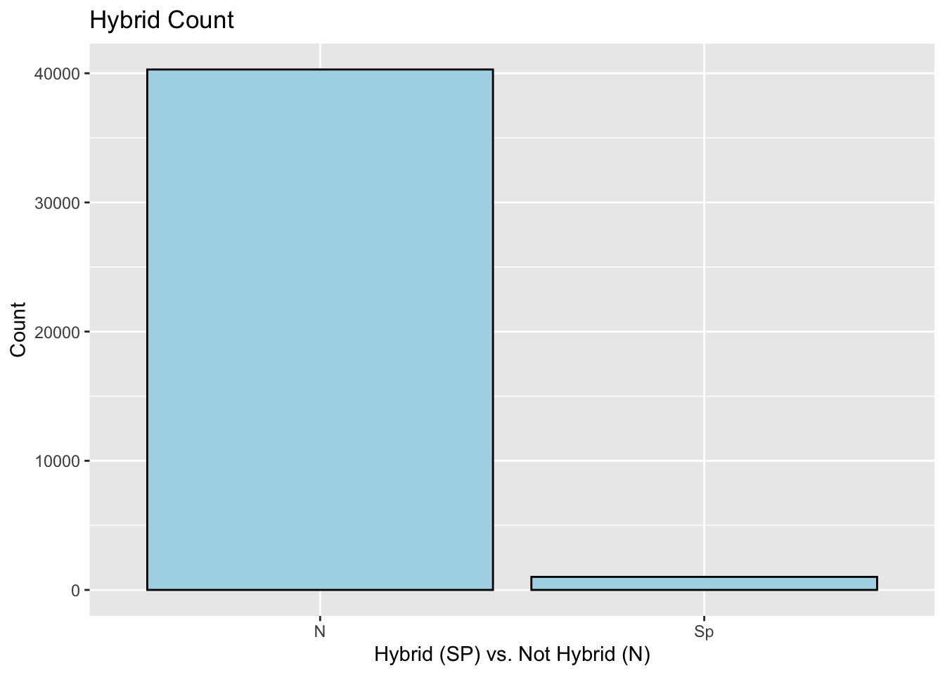
Here, we will look at the number of hybrids per taxon and per sex. In total there are 992 hybrids which is a small amount compared to the 40,312 that are not a hybrid. The ggplot is used to really accentuate the difference bewteen these two variables. The taxon EUL has the most hybrids which should be true as this is known as the hybrid species. There are 624 male hybrids and 368 female hybrids. My hypothesis was accepted, If hybrid Lemurs are born then they are more likely to be captive-born.

exploratory_data %>%
  count(hybrid)
# A tibble: 2 × 2
  hybrid     n
  <chr>  <int>
1 N      40292
2 Sp      1012
exploratory_data %>%
  group_by(taxon) %>%
  count(hybrid)
# A tibble: 29 × 3
# Groups:   taxon [27]
   taxon hybrid     n
   <chr> <chr>  <int>
 1 CMED  N       4015
 2 DMAD  N       2480
 3 EALB  N        161
 4 ECOL  N       1231
 5 ECOR  N       1050
 6 EFLA  N       1602
 7 EFUL  N        159
 8 EMAC  N        880
 9 EMON  N       1804
10 ERUB  N        688
# … with 19 more rows
exploratory_data %>%
  group_by(sex) %>%
  count(hybrid)
# A tibble: 6 × 3
# Groups:   sex [3]
  sex   hybrid     n
  <chr> <chr>  <int>
1 F     N      19991
2 F     Sp       358
3 M     N      20295
4 M     Sp       653
5 ND    N          6
6 ND    Sp         1
exploratory_data %>%
  ggplot() +
  geom_bar(mapping = aes(x = hybrid), color = "black", fill = "lightblue") +
  labs(title ="Hybrid Count", x = "Hybrid (SP) vs. Not Hybrid (N)", y = "Count")

  1. If Lemurs are mating it will more likely be in April and then the infants will be born around August and September.

According to this data, the conception month tends to be more around April, May, and June. Compared to the hypothesis of April, this wasn’t too off. The data also revealed that the infants are born in March, April, and May. The hypothesis predicted, August and September and this was way off. To find reasoning for this, I found the average expected gestation which was about 119 days. This tells us the period of developing inside the womb between conception and birth. 119 days is about 4 months so if conception occurred in April then the baby would be born around August which supports my hypothesis but does not hold true for the data.

exploratory_data %>%
  count(concep_month)
# A tibble: 13 × 2
   concep_month     n
          <dbl> <int>
 1            1  4925
 2            2  2238
 3            3  1973
 4            4  4014
 5            5  5182
 6            6  4189
 7            7  2154
 8            8  1762
 9            9  2078
10           10  2070
11           11  5932
12           12  4784
13           NA     3
exploratory_data %>%
  count(infant_dob_if_preg)
# A tibble: 490 × 2
   infant_dob_if_preg     n
   <date>             <int>
 1 1972-03-08             1
 2 1972-04-29             1
 3 1972-07-05             1
 4 1972-07-10             1
 5 1972-07-20             1
 6 1972-10-04             1
 7 1980-05-07             1
 8 1980-05-08             1
 9 1980-07-14             1
10 1981-03-06             1
# … with 480 more rows
exploratory_data %>%
  mutate(infant_dob_month = lubridate::month(infant_dob_if_preg)) %>%
  select(infant_dob_if_preg, infant_dob_month, everything()) %>%
  filter(!is.na(infant_dob_month)) %>%
  filter(!is.na(litter_size)) %>%
  group_by(infant_dob_month) %>%
  summarize(total_births = sum(litter_size))
# A tibble: 12 × 2
   infant_dob_month total_births
              <dbl>        <dbl>
 1                1           61
 2                2           62
 3                3          172
 4                4          121
 5                5          105
 6                6           71
 7                7           63
 8                8           24
 9                9           15
10               10           22
11               11            6
12               12           25
exploratory_data %>%
  summarize(avg_expected_gestation = mean(expected_gestation))
# A tibble: 1 × 1
  avg_expected_gestation
                   <dbl>
1                   120.

Inference

Here I’ll be using the “new” data which was unseen during the exploratory analysis seen earlier.

here are the hypotheses, I till be testing with this new data.

  1. If hybrid Lemurs are born then they are more likely to be captive-born rather than wild-born.

  2. If Lemurs are mating it will more likely be in April and then the infants will be born around August and September.

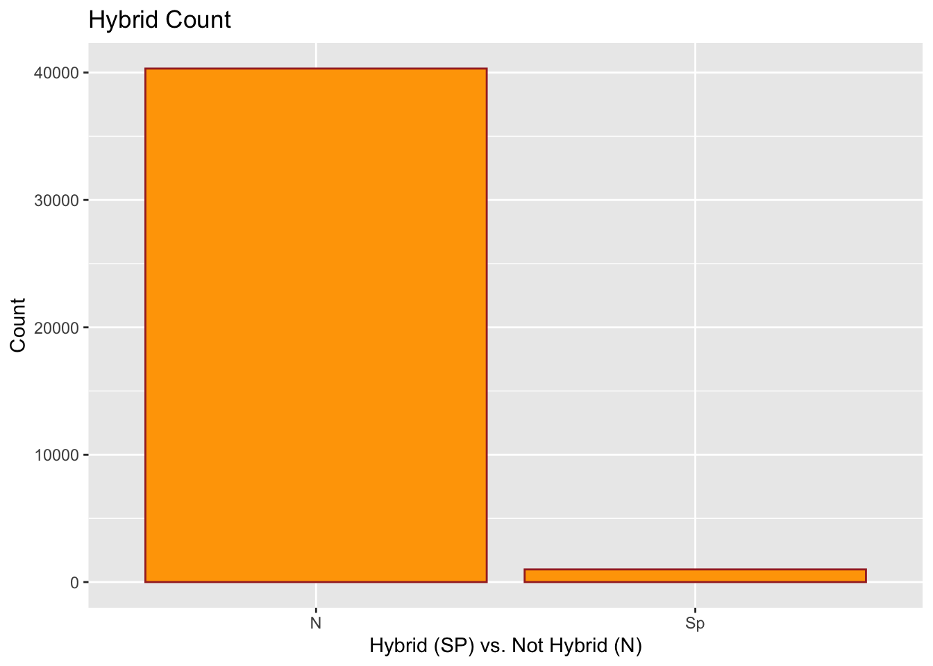
Using the new data, we will look at the number of hybrids per taxon and per sex. In total there are 1,034 hybrids which is a small amount compared to the 40,270 that are not a hybrid. The taxon EUL has the most hybrids which should be true as this is known as the hybrid species. There are 657 male hybrids and 377 female hybrids. My hypothesis was accepted, If hybrid Lemurs are born then they are more likely to be captive-born. Comparing this results to the exploratory data it is evident that the results have similar findings. These findings allow us to understand the data very well.

test_data %>%
  count(hybrid)
# A tibble: 2 × 2
  hybrid     n
  <chr>  <int>
1 N      40313
2 Sp       992
test_data %>%
  group_by(taxon) %>%
  count(hybrid)
# A tibble: 29 × 3
# Groups:   taxon [27]
   taxon hybrid     n
   <chr> <chr>  <int>
 1 CMED  N       4055
 2 DMAD  N       2597
 3 EALB  N        166
 4 ECOL  N       1236
 5 ECOR  N       1044
 6 EFLA  N       1615
 7 EFUL  N        169
 8 EMAC  N        854
 9 EMON  N       1841
10 ERUB  N        668
# … with 19 more rows
test_data %>%
  group_by(sex) %>%
  count(hybrid)
# A tibble: 5 × 3
# Groups:   sex [3]
  sex   hybrid     n
  <chr> <chr>  <int>
1 F     N      19847
2 F     Sp       361
3 M     N      20458
4 M     Sp       631
5 ND    N          8
test_data %>%
  ggplot() +
  geom_bar(mapping = aes(x = hybrid), color = "brown", fill = "orange") +
  labs(title ="Hybrid Count", x = "Hybrid (SP) vs. Not Hybrid (N)", y = "Count")

According to this new data, the conception month still tends to be more around April, May, and June. Compared to the hypothesis of April, this wasn’t too off. This new data also revealed that the infants are born in March, April, and May. The hypothesis predicted, August and September and this was way off. For this new data, the average expected gestation was also about 119 days. 119 days is about 4 months so if conception occurred in April then the baby would be born around August which supports my hypothesis but does not hold true for the data. These findings were exactly the same as the exploratory data findings. These findings allow us to understand the data very well.

test_data %>%
  count(concep_month)
# A tibble: 13 × 2
   concep_month     n
          <dbl> <int>
 1            1  4924
 2            2  2243
 3            3  2033
 4            4  4060
 5            5  5120
 6            6  4195
 7            7  2122
 8            8  1789
 9            9  2050
10           10  2015
11           11  5944
12           12  4805
13           NA     5
test_data %>%
  count(infant_dob_if_preg)
# A tibble: 488 × 2
   infant_dob_if_preg     n
   <date>             <int>
 1 1972-04-27             1
 2 1972-05-08             1
 3 1972-05-12             1
 4 1972-06-01             1
 5 1972-07-05             1
 6 1972-07-12             1
 7 1980-05-02             1
 8 1980-07-20             2
 9 1980-07-28             1
10 1980-08-16             1
# … with 478 more rows
test_data %>%
  mutate(infant_dob_month = lubridate::month(infant_dob_if_preg)) %>%
  select(infant_dob_if_preg, infant_dob_month, everything()) %>%
  filter(!is.na(infant_dob_month)) %>%
  filter(!is.na(litter_size)) %>%
  group_by(infant_dob_month) %>%
  summarize(total_births = sum(litter_size))
# A tibble: 12 × 2
   infant_dob_month total_births
              <dbl>        <dbl>
 1                1           81
 2                2           73
 3                3          164
 4                4           95
 5                5           90
 6                6           75
 7                7           59
 8                8           54
 9                9           15
10               10           20
11               11            7
12               12           30
test_data %>%
  summarize(avg_expected_gestation = mean(expected_gestation))
# A tibble: 1 × 1
  avg_expected_gestation
                   <dbl>
1                   119.

Conclusion

In conclusion, Lemurs are very interesting species. Lemurs are the most threatened group of mammals and are at risk of extinction. Lemurs are native to Madagascar which is located in the southwestern Indian Ocean. I’ve learned a lot about Lemurs through this report. My first hypothesis was If hybrid Lemurs are born then they are more likely to be captive-born rather than wild-born. In conclusion, my hypothesis was accepted, If hybrid Lemurs are born then they are more likely to be captive-born. My second hypothesis was If Lemurs are mating it will more likely be in April and then the infants will be born around August and September. In conclusion, the hypothesis was refuted but according to the expected gestation my hypothesis should have been on point. There are many other things to explore in this data set and many more interesting things to learn about Lemurs. This data comes from the Duke Lemur Center.